CellOrganizer for Galaxy
About CellOrganizer for Galaxy
CellOrganizer for Galaxy is a set of tools that enables users to train generative models of the cell from microscopy images, analyze trained generative models, and synthesize instances using CellOrganizer.
Using Galaxy
Galaxy is an open source, web-based platform for data intensive research.
There are many approaches to learning how to use Galaxy. To learn about Galaxy using the official tutorials, click here.
Using CellOrganizer for Galaxy
To start using CellOrganizer for Galaxy you can either
install the tools in your own Galaxy instance
use our public server
Installing local instance of CellOrganizer for Galaxy
Before you attempt to install the tools make sure to have
A working Galaxy instance. Installing Galaxy is beyond the scope of this document. Please refer to the official documentation to install an instance.
Matlab. Matlab should be installed in the same machine running Galaxy. Installing Matlab is beyond the scope of this document. Please refer to the official documentation to build an instance.
The Matlab binary must be in the $PATH of the user running Galaxy.
For example
``` ~ export PATH=$(PATH):/opt/matlab/bin ~ echo $PATH /usr/local/sbin:/usr/local/bin:/usr/sbin:/usr/bin:/sbin:/bin:/usr/games:/usr/local/games:/opt/matlab/bin
CellOrganizer must be downloaded into the system running Galaxy.
Its location should be set in an environment variable called $CELLORGANIZER. The environment variable needs to be accessible to the user running your Galaxy instance. Make sure the user running Galaxy has reading permissions on the CellOrganizer location.
``` ~ chown -R galaxy:galaxy /usr15/galaxy/cellorganizer-galaxy-tools-v2.9.0/cellorganizer3 ~ export CELLORGANIZER=/usr15/galaxy/cellorganizer-galaxy-tools-v2.9.0/cellorganizer3 ~ echo $CELLORGANIZER
/usr15/galaxy/cellorganizer-galaxy-tools-v2.9.0/cellorganizer3
To download CellOrganizer visit the official website. Please make sure the version of CellOrganizer you install matches the version of CellOrganizer for Galaxy.
Copy the CellOrganizer tools into the $GALAXY/tools. The variable $GALAXY, as explained in the official documentation, holds the location of your Galaxy instance.
Accessing the CellOrganizer for Galaxy public server
The CellOrganizer for Galaxy public server can be accessed at galaxy.compbio.cs.cmu.edu. This webserver is provided to grant access to CellOrganizer tools for users who do not have the resources to run the Matlab or Docker versions. It is provided at no charge for non-profit organizations.
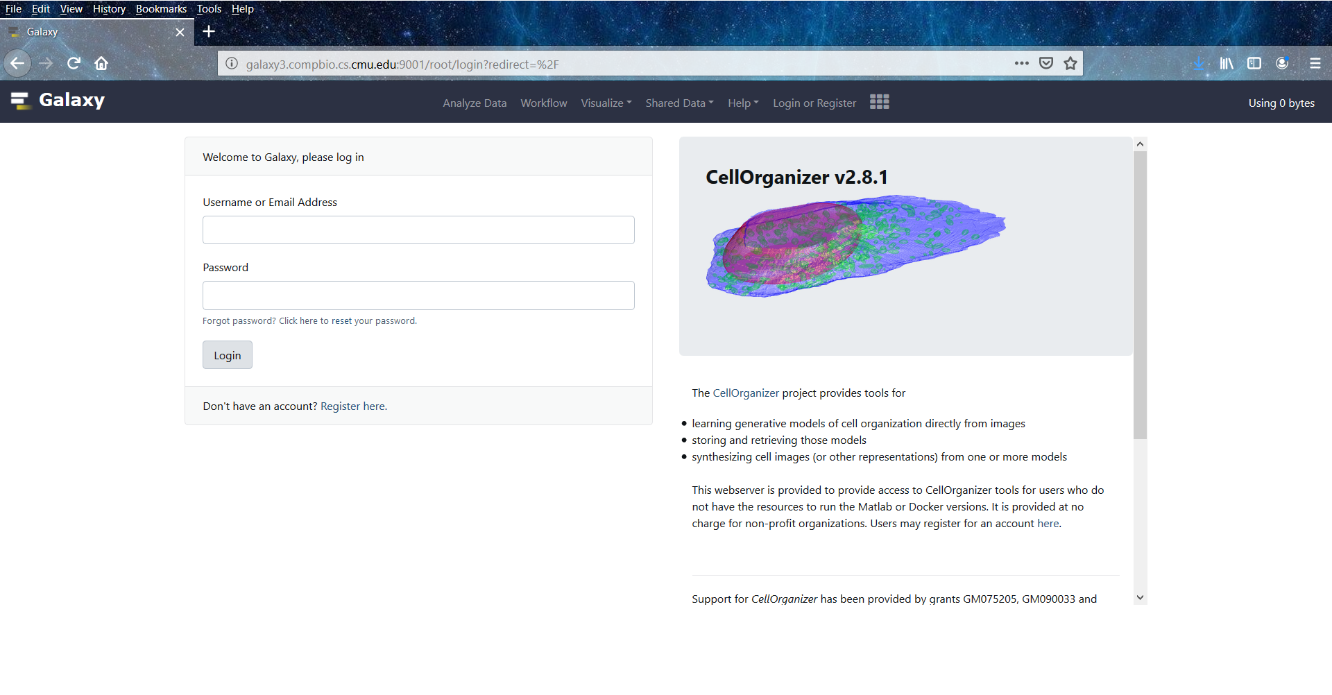
CellOrganizer for Galaxy public server welcome page.
Getting started
Essential features of CellOrganizer for Galaxy
Homepage
The homepage is divided into four parts
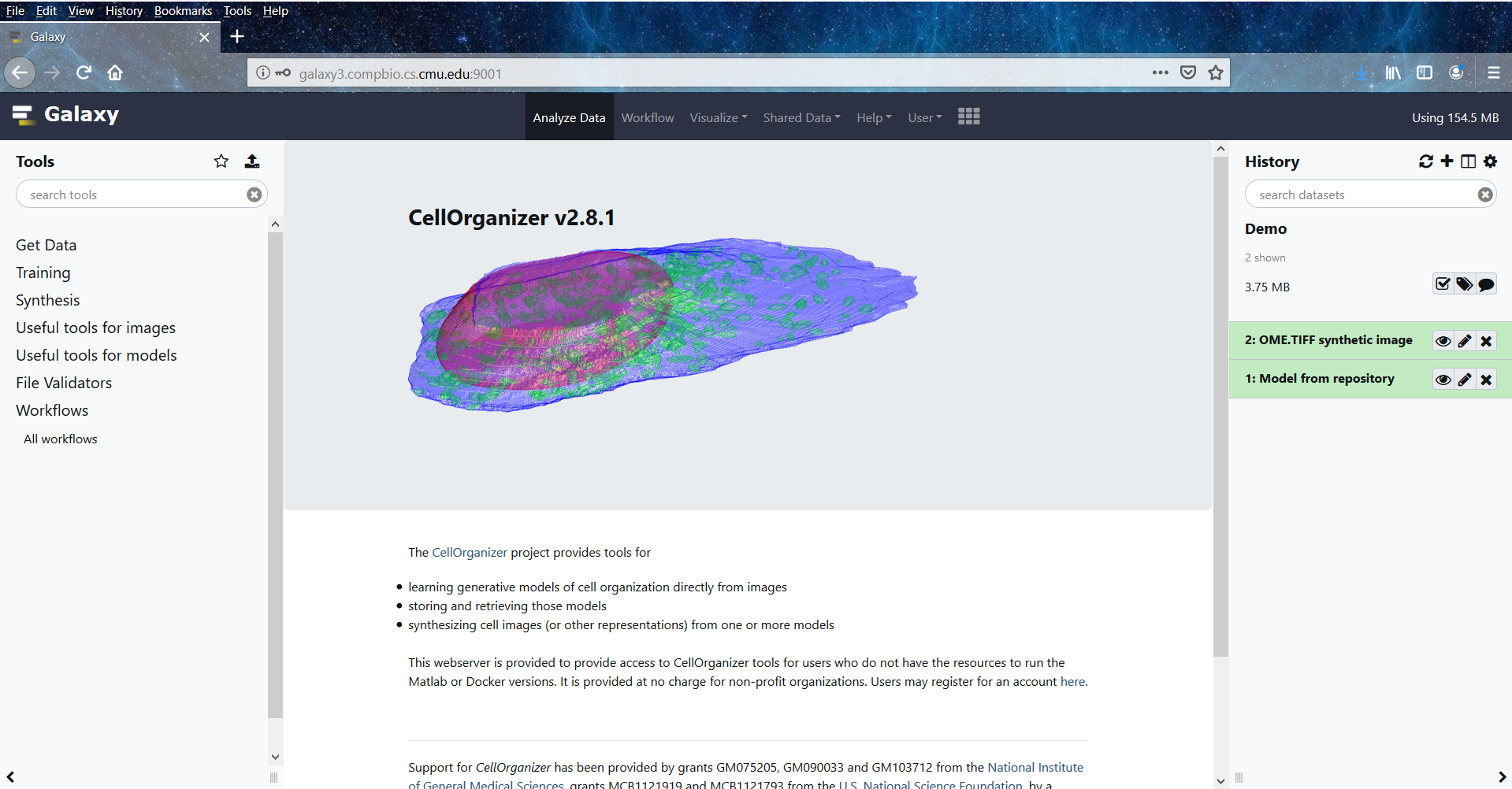
Navigation bar (top of the page)
Tools (left side of the page)
History (right side of the page)
Main Content window (center of the page)
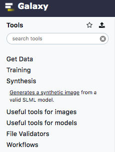
The Tools section lists all the tools that are available to the user. For user convenience, we have grouped the tools into six categories
Get Data (E.g under the Get Data section we have the following three tools)
Training
Synthesis
Useful tools for images
Useful tools for models
File Validators
The History window lists all the jobs that the user has submitted and indicates their respective statuses via color coding. Whenever the user executes a tool, it will submit a new job that will appear at the top of the History window as a rectangular box with a designed number and a descriptive name. The color of the box indicates the status of the corresponding job.
Gray means that the job has been submitted but not yet added to the job queue
Yellow means that the job has been submitted to the job queue
Red means that the job either exited before completion, or did not produce the expected output
Green means that the job ran successfully to completion and is ready to be viewed
The Main Content window is the CellOrganizer for Galaxy workspace. Once a tool or workflow (this term will be explained later) has been selected from the Tool Window, the user can specify the input parameters via the Main Content window.
List of Tools
The tools included in this release are
Upload file from your computer. This tool lets the user upload any file type to the Galaxy instance into the current workspace.
Imports image from a URL. This tool lets the user upload an OME.TIFF from URL and validate its metadata using BioFormats into the current workspace.
Imports model from the curated model repository. This tool lets the user to import a model from the CellOrganizer curated model repository into the current workspace.
Trains a generative model from a collection of OME.TIFFs.
Generates a synthetic image from a valid SLML model.
Exports a 2D synthetic image to a format that can be imported in VCell.
Generates a surface plot from a 3D OME.TIFF image.
Makes an RGB projection from an OME.TIFF.
Makes a projection from an OME.TIFF.
Print information about a generative model file.
Combine multiple generative model files into a single file.
Display shape space plot from a diffeomorphic or PCA model.
Validates an OME.TIFF.
Validates an SBML Level 3 instance.
Validates a Wavefront OBJ file.
Work Histories
Work Histories are Galaxy’s way of enabling users to create multiple isolated workspaces. You can think of your current Work History as your current workspace. At any point in time, your History window displays all the data you have either downloaded or produced in your current workspace.
Let’s say you download some data into your current Work History. That data is now accessible to tools in your Tools Window. You can apply any tool on that data, provided that it considers the data as valid input. The output of this operation will get saved to your current Work History, and now you can even apply tools to this newly accessible data as well.
If you now want to work on unrelated data, you can simply create a new Work History, switch your workspace to that newly created Work History, and work on that data without having to see the clutter of the previous workspace. Of course, you can always switch between Work Histories whenever you like.
Work Histories can be shared between Galaxy users, allowing them to see each other’s outputs/errors.
This table contains information about CellOrganizer demos. Click on the demo name to open the demo history in CellOrganizer for Galaxy tools.
We have provided links to sample histories constructed from CellOrganizer demos.
Demo |
Training |
Synthesis |
Other |
Deprecated |
|---|---|---|---|---|
True |
||||
True |
||||
True |
||||
True |
||||
True |
||||
True |
||||
True |
||||
True |
||||
True |
||||
True |
||||
True |
||||
True |
||||
True |
Plot |
|||
True |
||||
True |
Detailed information about Histories is beyond the scope of this document. To learn more about them, click here.
Jobs
Whenever you manage to execute a tool, you are essentially submitting a job to the server. And to execute a tool, you need to both provide the minimal set of inputs and to provide valid inputs. Whenever you click on one of the tools in the Tools Window, you should also see accompanying documentation in the Main Content window specifying what sort of inputs you need to provide to the tool.
Detailed information about Jobs is beyond the scope of this document. To learn more about them, click here.
Workflows
Workflows are Galaxy’s way of enabling users to automate particular pipelines (which can even be shared among users). You can also think of them as a means to construct more complex tools by piecing together simpler ones.
Let’s say you keep on repeating a certain procedure. You download data, run a tool on it to produce some output, then visualize the output. Each time you repeat the procedure, you first have to click on the tool to download data and fill up the necessary input values, then you have to wait for the data to be downloaded, then you have to click on the tool you wanted to run on the data and fill up the necessary input values, then … and so on. This is unnecessarily tedious.
Instead, we can streamline the procedure by linking the intermediate stages together via a Workflow. We get to fill up the necessary parameter settings that the intermediate stages require all at once. Then we can simply click run and wait for the final output.
We have provided links to sample workflows constructed using CellOrganizer for Galaxy tools.
Workflow Name |
|---|
Train-2D-diffeomorphic-framework-and-vesicular-pattern-model |
Detailed information about Workflows is beyond the scope of this document. To learn more about them, click here.
CellOrganizer for Galaxy Tutorial
Overview
Prerequisites for running CellOrganizer on Galaxy
Downloading Pre-Trained Model on Galaxy
Synthesizing synthetic images and SBML Instance from Model
Uploading and viewing your realistic geometry on CellBlender
Creating a Lotka-Volterra Simulation with your geometry
Prerequisites
Galaxy ( 2 options)
Installed version of Blender with the CellBlender package
Generating SBML Instance from Pretrained SPHARM-RPDM Model on Galaxy
Log in on Galaxy
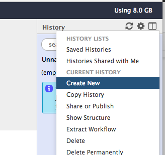
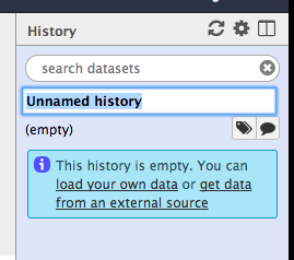
From the right panel (History panel) click on the “Gear Icon”
From the drop down menu click on “Create New”
To rename the history. Double click on “Unnamed history” and rename it to “SPHARM Model”. Then click enter.
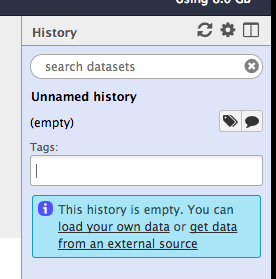
Annotate history. Click on the tag icon to add tags to this history. Add “train” and “vesicle” as tags. Click enter after each tag.
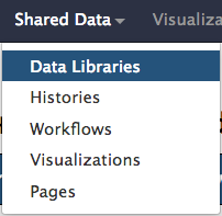
Import dataset from shared data. Click on “Shared Data” at the top of the screen then click on “Data Libraries” from the dropdown menu.
In the following page, follow the links for:
Click “Data Libraries” from the drop down menu.
Click on “Generative Models”
Click on “HeLa”
Click on “3D”
Click on “3D_HeLa_LAMP2_SPHARM_vesicle_model.mat”.
Then ticking off the box to the left of its name, then click on “To History” and select the history called “SPHARM Model”
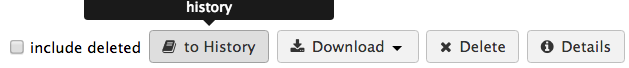
Then click on “to history” button in the top menu. A dialog window with appear with the current history on board pre-selected or you can create a new one as it gives you that option as well. * Click on the “import” button if your history is already pre-selected this will import both datasets into your history. Once the images are imported a green box in the top right corner will appear, click on it so it will take you to the history with the images imported
Or you can also click on the
 icon in the top left corner of the screen to return to the home page.
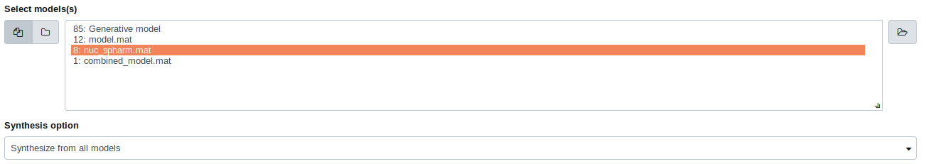
Then, click on “Synthesis” under the “Tools” menu, and follow the link to “Synthesize an instance from multiple models trained in CellOrganizer”
Select the model from the list and select “Synthesize from all models” as the synthesis option.
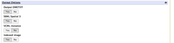
To save the output as an image and SBML mesh instance, click the YES button under Output Options for: OMETIFF, SBML Spatial 3, and Indexed Image
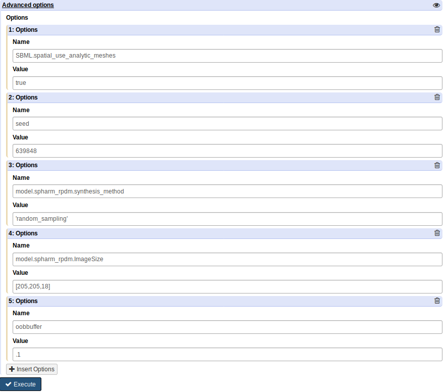
In the “Advanced Options”, match the following image:
Once all the information is complete click on the
 button, that will close the options panel. A green box will be displayed indicating that the demo is being run and a new item in the history will be added with the model ran.
- You should see your generated outputs in the right sidebar
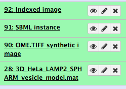
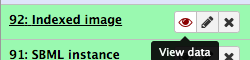
You can view the indexed image by clicking the eye icon next to the name
Importing Generated SBML instance into CellBlender
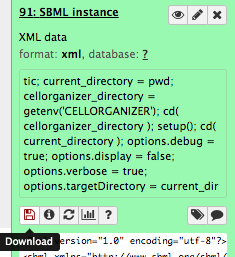
Download the SBML instance from Galaxy clicking the eye icon
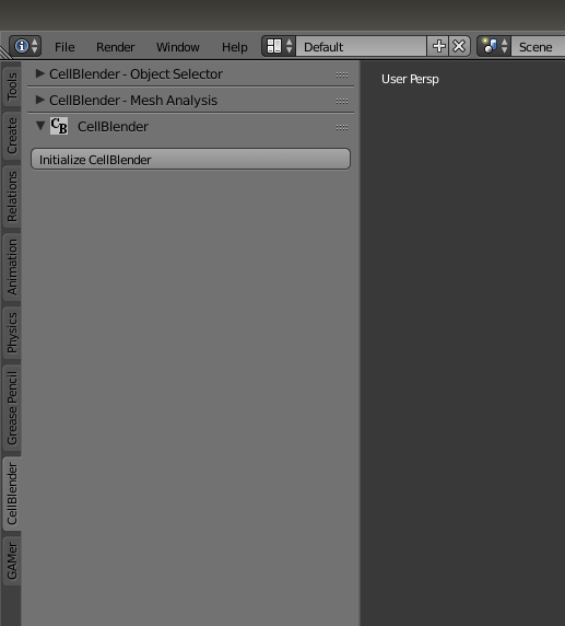
Next, open up Blender with CellBlender pre-installed. Initialize CellBlender.
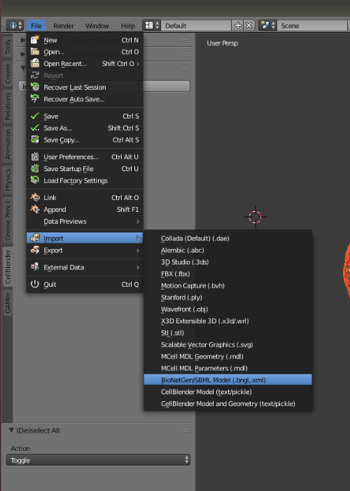
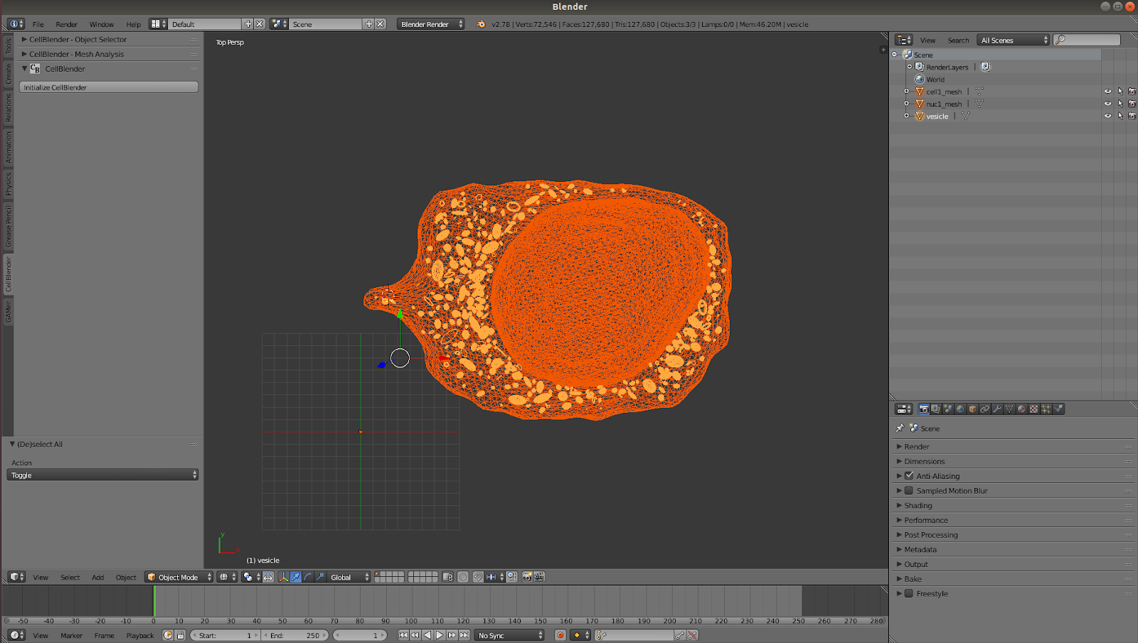
Import the downloaded SBML instance by going to: File > Import > BioNetGen/SBML Model(.bng, ./xml). You should now see your imported SBML instance. Use the scroll-pad and mouse to move around and investigate the geometry.
Create a Lotka-Volterra Simulation with our realistic geometry
Next step is to then import a .txt file, located at XXXXX, that includes the preset reactions for our simulation. Go to: File >Import >CellBlender Model(text/pickle)
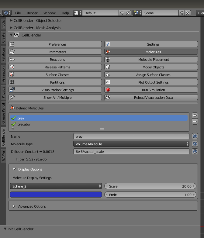
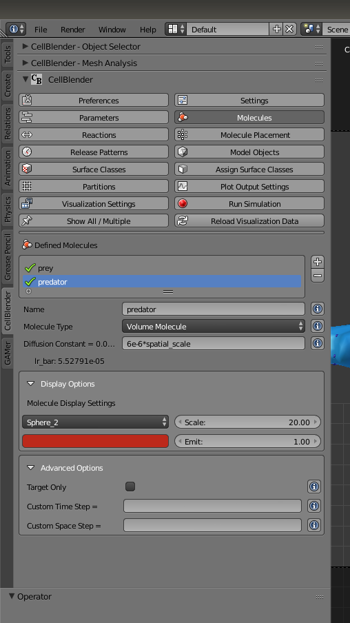
Next, we have to rescale and color our simulated particles. Under the “Molecules” button, set the scale of both “prey” and “predator” to 20.0. Set the color of “prey” to blue and “predator” to red.
Then, save the file as SPHARM_Model_Sim.blend. Next, you should see the Run button appear under the Run Simulation tab. Click that.
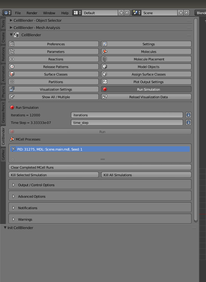
Note: It’s possible that the Run button doesn’t appear. This may be caused by the Mcell binary path not being set if not by default. Go to the Preferences tab under CellBlender and navigate to the option to set Mcell Binary Path. Depending on your device, this path should then be set to:
Linux: /home/[user]/blender-[version]/[version number]/scripts/addons/cellblender/bin/mcell
Windows: C:Users[user]AppDataRomaingBlender FoundationBlender[user]scriptsaddonscellblenderbinmcell
C:ProgramDataBlender FoundationBlender[user folder]scriptsaddonscellblenderbinmcell
with [user] and [version number] depending on your device.
This should produce a simulation similar to the one shown:
CellOrganizer for Galaxy Exercises
Input Type
In order to train a model, CellOrganizer requires you to have an image dataset. CellOrganizer provides sample image datasets for you to explore the software with. These sample image datasets are further described here. Once comfortable with the provided datasets, you are encouraged to upload your own image dataset for further computation given that all images in your dataset will meet certain parameters.
TIFF vs OME.TIFF
A TIFF image is a format that retains more pixels and provides a better resolution than a regular JPEG image. However, an OME.TIFF image retains the pixels of the image plus the metadata contained with it in an XML piece within the image.
What is an OME.TIFF format?
OME.TIFF is a bio-format that retains the pixels in multipage TIFF format, and simultaneously contains XML metadata because of the TIFF format it allows compatibility with many more applications. This image type combines both the TIFF format with the OME-XML format.
Image Specifications
- CellOrganizer training demos on MATLAB accept the following image file formats:
TIFF
OME-TIFF.
The minimum number of images to run a model is 20.
Images need to be processed as OME.TIFF format before they can be uploaded
Dataset if it is a collection should be a mix of HeLa Cells
Images must be static 2D or 3D dimensionality
Type (file): .mat, .OME.TIFF, .pdf, tabular, .tiff, .txt, vcml, xlsx, xml, zip
Import image from a URL - if images are in a repository just add the url for it.
Important
if you need to change the format of your images to OME.TIFF check here for more on what you will need to do. In most demos, CellOrganizer anticipates that you have a unique image dataset for each of the following three channels: cellular shapes, nucleoli, and proteins. You must set each of these variables individually and can choose to remove or add variables to comply with your own dataset. To set a variable, you are expected to either provide a list of the image filenames or a pattern of the image filenames. All images in the dataset are to be binarized and contrast – stretched prior to the main processing step.
Data Importing Exercises
Exercise 1. Importing image files that are already in CellOrganizer for Galaxy
Go to the navigation bar at the top of the homepage, click on “Shared Data”, and then choose “Data Libraries”.
Go to Images -> HeLa -> 2D -> LAMP2
Tick the box next to “LAMP2”.
Click on “To History”, select the history you would like to send the image dataset to, and then click “Import”.
Exercise 2. Importing a model that is already in CellOrganizer for Galaxy
Under the “Get Data” section of the Tools window, select “Downloads model from the curated model repository”.
Select the model you would like to import to the current history, and click “Execute”.
Exercise 3. Uploading image files / generative models from your computer
Under the “Get Data” section of the Tools window and select “Upload File from your computer”.
Click on “Choose local file” and then select image/model files that you wish to upload.
For every OMETIFF image that you upload, you should change the Type from “Auto-detect” to “tiff”. Similarly, for every model MAT-file that you upload, you should change the Type to “mat”. If all files that you are uploading have the same type, then you can simply use the “Type (set all)” option instead of having to make changes one at a time.
Click on “Start”.
Model Training Exercises
Exercise 4. Train a shape space model for 2D cell and nuclear shape using the PCA approach
Create a new history if desired.
Import the “2D HeLa LAMP2” image dataset from “Shared Data” (See Exercise 1), and create a dataset collection called “2D HeLa LAMP2” from these image files (See section Creating a collection from datasets in your history in link).
Under the “Training” section of the Tools window, select “Trains a generative model”.
Directly under “Choose a data set for training a generative model”, there should be two icons. If you hover your cursor over them, one says “Multiple datasets” and the other says “Dataset collections”. Click on the icon for “Dataset collections” and select the “2D HeLa LAMP2” dataset collection as the input dataset collection.
Select the following settings
Select the cellular components desired for modeling: Nuclear and cell shape (framework)
Dimensionality: 2D
Nuclear shape model class: Framework
Nuclear shape model type: PCA
Cell shape model class: Framework
Cell shape model type: PCA
Under the “Advanced options” section, click “Insert Options”, and then fill in latent_dim for “Name” and 15 for “Values”.
Fill in 2D-HeLa-LAMP2-PCA under “Provide a name for the model”.
Do not change any other default settings, and click “Execute”.
Exercise 5. Train a model for punctate organelles (e.g. vesicles) from a subset of the 3D HeLa LAMP2 collection
Create a new history if desired.
Import the “3D HeLa LAMP2” dataset collection from “Shared Data” (See Exercise 1).
Under the “Training” section of the Tools window, select “Trains a generative model”.
Select the “3D HeLa LAMP2” dataset as the input dataset. And select the following settings
Select the cellular components desired for modeling: Nuclear shape, cell shape and protein pattern
Dimensionality: 3D
Protein model protein location: Nucleus and cytoplasm
Fill in 3D-HeLa-LAMP2-classic under “Provide a name for the model”.
Do not change any other default settings, and click “Execute”.
Exercise 6. Train a diffeomorphic shape space model for cell and nuclear shape from a subset of the 3D HeLa LAMP2 collection
Create a new history if desired.
Import the “3D HeLa LAMP2” dataset collection from “Shared Data” (See Exercise 1).
Under the “Training” section of the Tools window, select “Trains a generative model”.
Select the “3D HeLa LAMP2” dataset as the input dataset. And select the following settings
Select the cellular components desired for modeling: Nuclear and cell shape (framework)
Dimensionality: 3D
Nuclear shape model class: Framework
Nuclear shape model type: Diffeomorphic
Cell shape model class: Framework
Cell shape model type: Diffeomorphic
Fill in 3D-HeLa-LAMP2-diffeo under “Provide a name for the model”.
Do not change any other default settings, and click “Execute”.
Model Synthesis Exercises
Exercise 7. Synthesize an image from an existing model
Create a new history if desired.
Import the “3D HeLa vesicle model of mitochondria” and the “2D HeLa vesicle model of nucleoli” from the curated model repository (See Exercise 2).
Under the “Synthesis” section of the Tools window, select “Generates a synthetic image …”
Select the “3D HeLa vesicle model of mitochondria” as the input model, and select the “Synthesis option” as “Synthesize from all models”.
Click “Execute”.
Repeat steps 3-5, but this time select the “2D HeLa vesicle model of nucleoli” as the input model, and select the “Synthesis option” as “Synthesize nuclear and cell membrane (framework)”.
Model Combination Exercises
Exercise 8. Combine the Nuclear shape component of one model with the Cell shape component of another model into a single model
Select or create a history that contains at least two models. For this exercise, we will use the models “2D HeLa - medial axis and ratio models of the cell and nucleus - vesicle model of endosomes” and “2D HeLa - medial axis and ratio models of the cell and nucleus - vesicle model of lysosomes” from the curated model repository (See Exercise 2).
Under “Useful tools for models” select “Combine multiple generative model files into a single file”.
Click on “Insert Models” twice to open two model selection sections.
In the first model selection section, select the model whose Nuclear shape component we want to use.
In the second model selection section, select the model whose Cell shape component we want to use.
(Optional) If you want to add additional documentation to the combined model, click “Insert Documentation”. Under the “Name” section, fill in (without quotes) the word ‘documentation’. Under the “Values” section, fill in any additional information you want to store within the model and enclose that information in quotes (E.g. ‘This model was created by combining model A’s Nuclear shape component with model B’s Cell shape component’).
Click “Execute”. The tool will now produce a new model with the Nuclear shape component of the first model, and the Cell shape component of the second model.
Exercise 9. Combine the Nuclear shape and Cell shape components of one model with the Protein distribution component of another model into a single model
Select or create a history that contains at least two models. For this exercise, we will use the models “2D HeLa - medial axis and ratio models of the cell and nucleus - vesicle model of endosomes” and “2D HeLa - medial axis and ratio models of the cell and nucleus - vesicle model of lysosomes” from the curated model repository (See Exercise 2).
Under “Useful tools for models” select “Combine multiple generative model files into a single file”.
Click on “Insert Models” thrice to open three model selection sections.
In both the first and second model selection sections, select the model whose Nuclear shape and Cell shape components we want to use.
In the third model selection section, select the model whose Protein distribution component we want to use.
(Optional) If you want to add additional documentation to the combined model, click “Insert Documentation”. Under the “Name” section, fill in (without quotes) the word ‘documentation’. Under the “Values” section, fill in any additional information you want to store within the model and enclose that information in quotes (E.g. ‘This model was created by combining model A’s Nuclear shape and Cell shape components with model B’s Protein distribution component’).
Click “Execute”. The tool will now produce a new model with the Nuclear shape and Cell shape components of the first model, and the Protein distribution component of the third model.