Tutorial: CellOrganizer in 45 Minutes¶

Publications¶

cellorganizer.org/Publications/

Software¶

cellorganizer.org - Current CellOrganizer distribution

Other Software¶

ImageJ - This is great software for viewing your images and those synthesized from CellOrganizer. This tutorial uses ImageJ in some spots.

Image Databases¶

• www.openmicroscopy.org/
• www.cellimagelibrary.org
• www.proteinatlas.org/subcellular
• murphylab.web.cmu.edu/data/

Step 0: Download the most recent version of CellOrganizer¶

The software can be downloaded from cellorganizer.org, unzip it, and copy the resulting folder into the “Documents” → “MATLAB” directory.

Step 1: Add the CellOrganizer directory to the Path¶

You should see the folder appear in the “Current Folder” in MATLAB on the left side. If it doesn’t, make sure that your file path is “Users” → your user name → “Documents” → “MATLAB”.

Step 2: Get your images on the same computer¶

If you don’t have your own images, you can download some samples here, or you can type get_murphylab_image_collections. (Note:: The whole collection is 2.0 GB.) These are 3D HeLa images with a nuclear stain (channel 0), cell stain (channel 1) and protein stain (channel 2). The tagged protein is lamp2, a lysosomal protein. Unzip the file to some directory of your choice. Optionally, to decrease training time, set aside 10 to 15 images that will not be used.

Step 0: Create a “scratch” script¶

This will keep track of what you have done so far and provide a resource for later use of CellOrganizer. Click “File” → “New” → “New Script”, and save your file as tutorial_train.m (making sure that the file is saved to the “Documents” → “MATLAB” path, but not inside the “cellorganizer” folder). Instead of typing the following commands into the Command Window, type (or copy and paste) them into the script that you just created.

Step 1: Create variables containing your images¶

There are three ways to do this depending on how you have stored your images, each of which has its own strengths: string wildcards, a cell array of file paths, and a cell array of function handles.

To make life easier in the future, start by defining a variable that contains the path to the images’ directory. Something like this:

img_dir = '/Users/greg/Desktop/LAM';

nuc_img_paths = [img_dir '/cell*_ch0_t1.tif'];
cell_img_paths = [img_dir '/cell*_ch1_t1.tif'];
prot_img_paths = [img_dir '/cell*_ch2_t1.tif'];

for i = 1:15
        nuc_img_paths{i} = [img_dir '/cell' num2str(i) '_ch0_t1.tif'];
        cell_img_paths{i} = [img_dir '/cell' num2str(i) '_ch1_t1.tif'];
        prot_img_paths{i} = [img_dir '/cell' num2str(i) '_ch2_t1.tif'];
end

for i = 1:15
        nuc_img_paths{i} = @() ml_readimage([img_dir '/cell' num2str(i)...
        '_ch0_t1.tif']);
        cell_img_paths{i} = @() ml_readimage([img_dir '/cell' num2str(i)...
        '_ch1_t1.tif']);
        prot_img_paths{i} = @() ml_readimage([img_dir '/cell' num2str(i)...
        '_ch2_t1.tif']);
end

Step 2: Setup the option structure¶

The option structure tells CellOrganizer how you want to build a model, and allows for option input. Most of the options have default values, so we don’t have to set them manually for this tutorial. However, we do need to know the pixel resolution of the images and a filename to save the resulting model in. To define the appropriate options, we create a struct variable called train_options and set fields accordingly:

%this is the pixel resolution in um of the images
train_options.model.resolution = [0.049, 0.049, 0.2000];

%this tells CellOrganizer what channels to build models for
train_options.train.flag = 'all';

%this is the filename to be used to save the model in
train_options.model.filename = 'model.mat';

The option train.filename defines where the .mat file containing the resulting model should be saved. By setting train_options.train.flag to 'all' we specify training a model that trains a nuclear shape, cell shape and protein distribution model. We can also specify the train flag as 'framework' to train just a nuclear shape and cell shape model (and we would therefore no longer need to provide protein images), or set the flag to 'nuc' and just train a nuclear shape model (and not have to provide cell shape images).

So far we have the bare minimum requirements for setting up a model. We will set one more option to speed up the tutorial.:

train_options.model.downsampling = [4,4,1];

This downsamples our input images by 4 in the X and Y dimensions, decreasing the memory used for the tutorial.

Step 2.5: Add a model type¶

We also need to specify what type of model we want to train. We do this by adding additional lines to the options structure:

train_options.nucleus.type = 'cylindrical_surface';
train_options.cell.type = 'ratio';
train_options.protein.type = 'vesicle';
train_options.debug = true;

Now that we have everything together, we can train the model:

img2slml('3D', nuc_img_paths, cell_img_paths, prot_img_paths, train_options);

If your model building options don’t require one of the image types (e.g., the protein images are not needed in this case), you can just use empty brackets:

img2slml('3D', nuc_img_paths, cell_img_paths, [], train_options);

(make sure that your inputs to img2slml correspond to your setting of train.flag)

Step 3: Run your script¶

Press the play button on the top of the Matlab window or type the name of your script into the Command Window. If you used a lot of images or did not aggressively downsample your images this may take some time.

Step 4: Your model¶

Now that your run of CellOrganizer has completed without error, you should have a .mat file named model.mat in the directory in which you ran the code. Congratulations, you made it! If you load that file into your Workspace you’ll see that this is another struct with fields. This is the model of your cell images. You’ll notice that it’s a lot smaller in file size than the collection of source images you used to train it. Take some time to explore these fields.

Step 0: Create a “scratch” script¶

Here we create a new script and call it tutorial_synthesis.m.

Step 1: Setup the model and option inputs¶

Start by defining two variables: a cell-array containing the path to the model you created in the Training section, and a new option structure (different from the one used for learning). If you followed the instructions in the Training section, then you should be able to create a variable using the same path as in Step 2 of Training.:

model_path = {'model.mat'};

Alternatively you can generate images from one of the models provided in the CellOrganizer distribution, such as the model of the lysosomal protein LAMP2 in HeLa cells:

model_path = {'./cellorganizer-v2.5/models/3D/lamp2.mat'};

The option structure is set up similarly to that in Training. Here we create a new struct called synth_options and define where we want the images to be saved, a prefix for the saved files and the number of images desired:

%save into the current directory
synth_options.targetDirectory = './';

synth_options.prefix = 'synthesis_tutorial';

%generate two images
synth_options.numberOfSynthesizedImages = 2;

Step 2: Controlling the random seed (optional)

CellOrganizer generates synthetic images by randomly drawing parameter values from the distributions contained in the specific model. The random numbers are provided by the Matlab rand function, and the specific sequence of random numbers the program will get when it calls rand can be controlled by specifying what is termed a random seed (which can be any number) using the rng function:

rng(666);

If we do this, the specific images that CellOrganizer will generate will be the same each time our script is run. If we don’t, the images will be based upon the current state of the random number generator, and we may get different images each time we run the script.

Now that we have everything set up, we can generate an image or two!

Step 3: Synthesize¶

As the last line of our script, we call slml2img.m:

slml2img(model_path, synth_options);

Save your file and run it. This may take a while, especially if you have decided to generate many images.

Step 4: Check out your images¶

Now that the image generation is completed, you can view them. In the current directory you should see a folder named “synthesis_tutorial”, and in that should be two directories, “cell1” and “cell2”, each of which contain images corresponding to each channel drawn from the model you trained in the Training section. While these images can be opened in ImageJ, we are going to demonstrate two useful tools in CellOrganizer that we frequently use to explore our synthesized images.

First we’re going to create an indexed image by combining output images.:

%read in each image to a variable
im_cell = ml_readimage('<path to cell image>');
im_dna = ml_readimage('<path to nucleus image>');
im_prot = ml_readimage('<path to protein image>');

%create an empty image
im_indexed = zeros(size(im_cell));

%Set the cell shape, nuclear shape and protein shape values to 1,2,3 respectively
im_indexed(im_cell>0) = 1;
im_indexed(im_dna>0) = 2;
im_imdexed(im_prot>0) = 3;

Now that we have an image, we can view it with the function img2vol (after downsampling it by a factor of two in X, Y and Z:

figure, img2vol(ml_downsize(im_indexed, [2,2,2]));

Congratulations! You have created a synthetic cell geometry!

Background¶

Upon exposure to Bafilomycin A1, microtubule associated protein light chain 3 (LC3) localizes into autophagosomes for degradation and forms punctate structures.

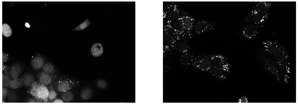
Images of eGFP-LC3 tagged RT112 cells at 40x under normal conditions (left) and in a 50uM Bafilomycin condition (right).

Let’s say we are curious as to how the number of autophagosomes changes with Bafilomycin concentration. Given a collection of images under different concentrations we can segment out the cell shapes and train a model for the cells contained in each image. It just so happens that we have already done that, and the models and associated drug concentrations, can be found here.

That .mat file has two variables saved in it. One is a list of drug micromolar concentrations, and the other is a list of models trained with images of cells at those concentrations (like the above two images). For each model, we’re going to plot the number of autophagosomes versus the Bafilomycin concentration.

Step 0: Create another “scratch” script¶

Lets call this one plotObjsByModel.m

Step 1: Load the model data into the workspace¶

Load the .mat file you downloaded into the Workspace by double clicking on it. You should see two variables, conc, and models. These are the variables that contain the drug concentrations and trained CellOrganizer models of cells exposed to Bafilomycin at those concentrations. You can access the first model by typing models{1}, the second model by models{2} and so on. You will see that there are a lot of components to these models, but we’re just interested in the number of objects under each conditions.

Step 2: Plot the average number of autophagosomes for each model¶

We must access the component of the model that contains the distribution for the number of objects. We can access that in the first model with:

models{1}.proteinModel.objectModel.numStatModel

The output should be:

ans =

name: 'gamma'
alpha: 2.7464
beta: 19.291

This means that the distribution over the number of objects contained in the cells that were used to train this model is modeled as a gamma distribution with two parameters, alpha, and beta. It just so happens that the average of a gamma distribution is the product of these two parameters. Let’s write a loop to get the average number of autophagosomes from each model:

for i = 1:length(models)
        numObjsModel = models{i}.proteinModel.objectModel.numStatModel;
        avgObjects(i) = numObjsModel.alpha*numObjsModel.beta;
end

Now we simply plot the number of objects versus drug concentration. Here we will use a semilog plot to make visualization easier:

semilogx(conc, avgObjects, 'linestyle', 'none', 'marker', '.', 'markersize', 10)
ylabel('Mean Number of Objects Per Model')
xlabel('[Bafilomycin A1] (uM)')